Web Scraping for Machine Learning

You can see the full guide on our blog.

Project requirements

$ python3 -m pip install requests_html beautifulsoup4

$ python3 -m pip install pandas numpy matplotlib seaborn tensorflow scikit-learn keras

Extracting the data

If we’re looking at machine learning projects, Jupyter Notebook is a great choice as it’s easier to run and rerun a few lines of code. Moreover, the plots are in the same Notebook.

Begin with importing required libraries as follows:

from requests_html import HTMLSession
import pandas as pd

For web scraping, we only need Requests-HTML. The primary reason is that Requests-HTML is a powerful library that can handle all our web scraping tasks, such as extracting the HTML code from websites and parsing this code into Python objects. Further benefits come from the library’s ability to function as an HTML parser, meaning collecting data and labeling can be performed using the same library.

Next, we use Pandas for loading the data in a DataFrame for further processing.

In the next cell, create a session and get the response from your target URL.

url = 'https://finance.yahoo.com/quote/AAPL/history?p=AAPL&guccounter=1&period1=1556113078&period2=1713965616'
session = HTMLSession()
r = session.get(url)

After this, use XPath to select the desired data. It’ll be easier if each row is represented as a dictionary where the key is the column name. All these dictionaries can then be added to a list.

rows = r.html.xpath('//table/tbody/tr')
symbol = 'AAPL'
data = []
for row in rows:
    if len(row.xpath('.//td')) < 7:
        continue
    data.append({
        'Symbol':symbol,
        'Date':row.xpath('.//td[1]/text()')[0],
        'Open':row.xpath('.//td[2]/text()')[0],
        'High':row.xpath('.//td[3]/text()')[0],
        'Low':row.xpath('.//td[4]/text()')[0],
        'Close':row.xpath('.//td[5]/text()')[0],
        'Adj Close':row.xpath('.//td[6]/text()')[0],
        'Volume':row.xpath('.//td[7]/text()')[0]
    }) 
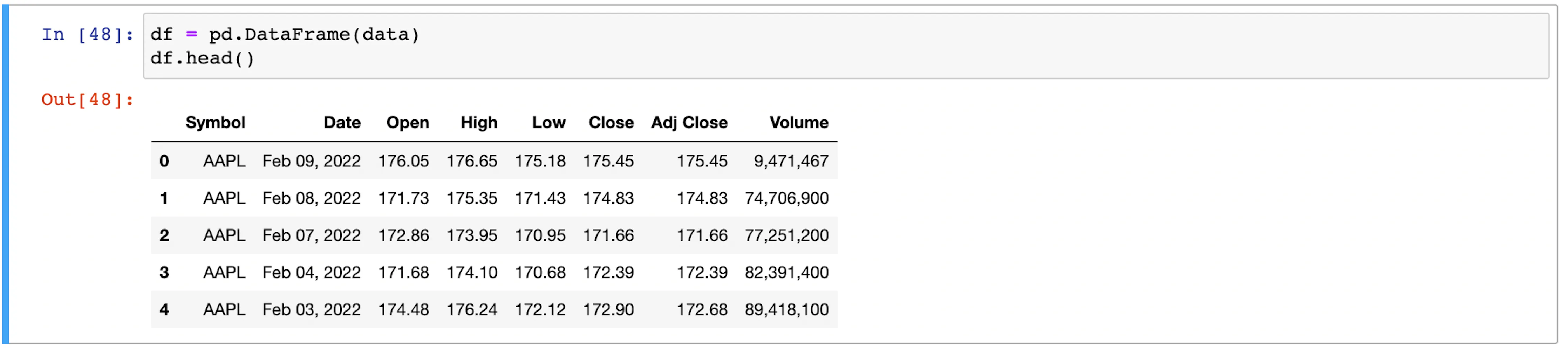
df = pd.DataFrame(data)

The results of web scraping are being stored in the variable data. To understand why such actions are taken, we must consider that these variables are a list of dictionaries that can be easily converted to a data frame. Furthermore, completing the steps mentioned above will also help to complete the vital step of data labeling.

The provided example’s data frame is not yet ready for the machine learning step. It still needs additional cleaning.

Cleaning the data

Now that the data has been collected using web scraping, we need to clean it up. The primary reason for this action is uncertainty whether the data frame is acceptable; therefore, it’s recommended to verify everything by running df.info().

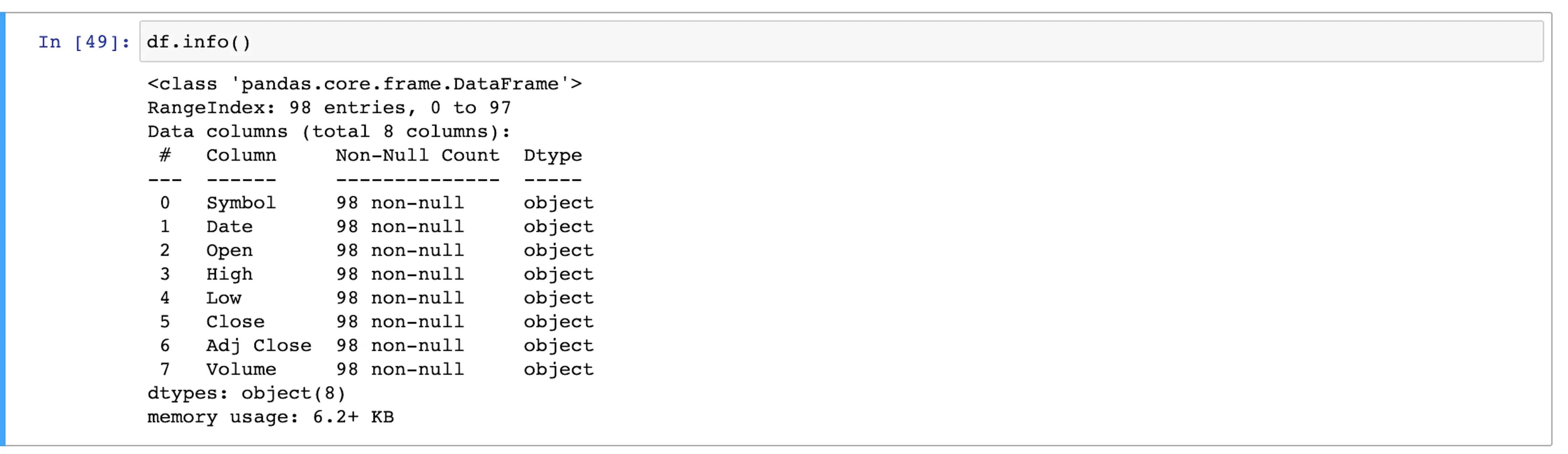
As evident from the above screen-print, all the columns have data type as object. For machine learning algorithms, these should be numbers.

Dates can be handled using Pandas.to_datetime. It’ll take a series and convert the values to datetime. This can then be used as follows:

df['Date'] = pd.to_datetime(df['Date'])

The issue we ran into now is that the other columns were not automatically converted to numbers because of comma separators.

Thankfully, there are multiple ways to handle this. The easiest one is to remove the comma by calling str.replace() function. The astype function can also be called in the same line which will then return a float.

str_cols = ['High', 'Low', 'Close', 'Adj Close', 'Volume']
df[str_cols]=df[str_cols].replace(',', '', regex=True).astype(float)

Finally, if there are any None or NaN values, these can be deleted by calling the dropna().

df.dropna(inplace=True)

As the last step, set the Date column as the index and preview the data frame.

df = df.set_index('Date')
df.head()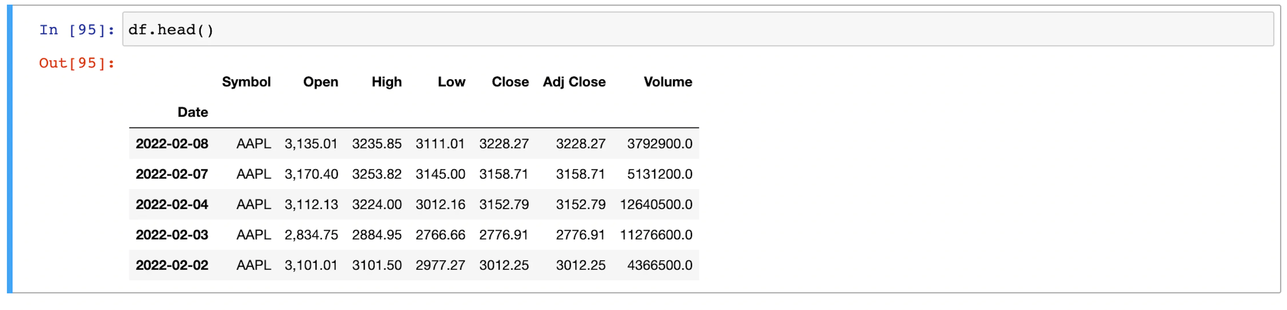

The data frame is now clean and ready to be sent to the machine learning model.

Visualizing the data

Before we begin the section on machine learning, let’s have a quick look at the closing price trend.

First, import the packages and set the plot styles:

import matplotlib.pyplot as plt
import seaborn as sns
sns.set_style('darkgrid')
plt.style.use('ggplot')

Next, enter the following lines to plot the Adj Close, which is the adjusted closing price

plt.figure(figsize=(15, 6))
df['Adj Close'].plot()
plt.ylabel('Adj Close')
plt.xlabel(None)
plt.title('Closing Price of AAPL')
plt.show()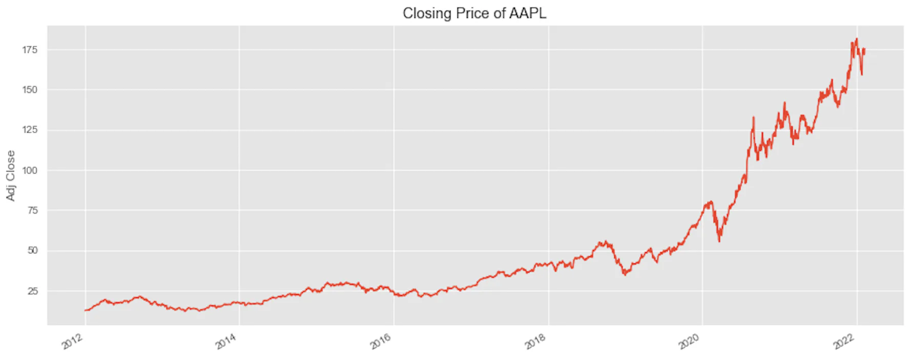

Preparing data for machine learning

The first step to machine learning is the selection of features and values we want to predict.

In this example, the “Adjusted Close” is dependent on the “Close” part. Therefore, we’ll ignore the Close column and focus on Adj Close.

The features are usually stored in a variable named X and the values that we want to predict are stored in a variable y.

features = ['Open', 'High', 'Low', 'Volume']
y = df.filter(['Adj Close'])

The next step we have to consider is feature scaling. It’s used to normalize the features, i.e., the independent variables. Within our example, we can use MinMaxScaler. This class is part of the preprocessing module of the Sci Kit Learn library.

First, we’ll create an object of this class. Then, we’ll train and transform the values using the fit_transform method as follows:

from sklearn.preprocessing import MinMaxScaler
scaler = MinMaxScaler()
X = scaler.fit_transform(df[features])

The next step is splitting the data we have received into two datasets, test and training.

The example we’re working with today is a time-series data, meaning data that changes over a time period requires specialized handling. The TimeSeriesSplit function from SKLearn’s model_selection module will be what we need here.

from sklearn.model_selection import TimeSeriesSplit
tscv = TimeSeriesSplit(n_splits=10) 
for train_index, test_index in tscv.split(X):
    X_train, X_test = X[train_index], X[test_index]
     y_train, y_test = y.iloc[train_index], y.iloc[test_index]

Our approach for today will be creating a neural network that uses an LSTM or a Long Short-Term Memory layer. LSTM expects a 3-dimensional input with information about the batch size, timesteps, and input dimensions. We need to reshape the features as follows:

X_train = X_train.reshape(X_train.shape[0], 1, X_train.shape[1])
X_test = X_test.reshape(X_test.shape[0], 1, X_test.shape[1])

Training the model and predictions

We’re now ready to create a model. Import the Sequential model, LSTM layer, and Dense layer from Keras as follows:

from keras.models import Sequential
from keras.layers import LSTM, Dense

Continue by creating an instance of the Sequential model and adding two layers. The first layer will be an LSTM with 32 units while the second will be a Dense layer.

model = Sequential()
model.add(LSTM(32, activation='relu', return_sequences=False))
model.add(Dense(1))
model.compile(loss='mean_squared_error', optimizer='adam')

The model can be trained with the following line of code:

model.fit(X_train, y_train, epochs=100, batch_size=8)

While the predictions can be made using this line of code:

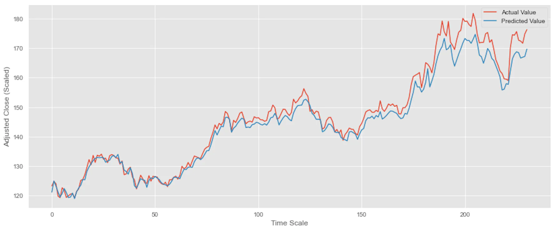
y_pred= model.predict(X_test)

Finally, let’s plot the actual values and predicted values with the following:

plt.figure(figsize=(15, 6))
plt.plot(y_test.values, label='Actual Value')
plt.plot(y_pred, label='Predicted Value')
plt.ylabel('Adjusted Close (Scaled)')
plt.xlabel('Time Scale')
plt.legend()